Capstone: Machine Learning for Active Shooter events
Using Batch Spectrograms and Image Recognition
Project Specifications
Some Notes about capstone
This project was built mainly using Python, Python packages, TensorFlow, and Raspberry Pi. All students in the Electrical Engineering program at Texas A&M must complete a sponsored 2-semester capstone program. This is a very involved program usually involving 30-40 hrs of work each week. Each week included constant reporting to supervisors, oral presentations, and laboratory work. While the project is a group project, here I talk about my work on the project, and how I helped the other members when needed. I received no help with the machine learning aspects of this project.
FSR (Functional System Requirements)
This is a shortened list since the actual FSR is over 20 pages long. I also list the FSR of the other components since it is relevant to how I work with other systems.
There were 3 members and therefore 3 main subsystems.
- Machine Learning Inference System
- Sound Location System
- End User Screen and Transmission System
The Requirements:
- The ASD (Active Shooter Detector) must differentiate when there is gunfire or not.
- The ASD must source the location of said noise in 3D space.
- The ASD must relay metrics from 1 and 2 to an officer through a screen.
- The ASD must be mounted on a rover and capable of rotational and/or translational movement, controlled by the screen mentioned in 3.
ICD (Interface Control Document)
This is a graphical representation. The actual ICD specifies all of the possible standards and interconnection issues for each interface and is over 20 pages long.
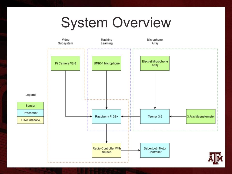
System Overview: note interaction with other subsystems
Research
Data collection
My sponsor used the UMK-1 microphone to record gunfire at a local gun-range with various kinds of weapons. The reason that UMK-1 was chosen was because of its higher recording Frequency response compared to other USB plugs in microphones.
This batch of .wav files was then combined with a large open-source of .wav files which were an accumulation of “loud” sounds. I say “loud” because there was not a defined limit as to what “loud” meant.
The Model
The next step was to pick a model for audio inference. Here we had to make a tough choice. Unlike common Linear Regressions, Audio has interesting constraints. For starters, it has more dimensionality, which restricts augmentation. How do you skew, flip, or stretch Audio without losing temporal fidelity?
The LSTM( Long and Short Term Memory) or BERT(Bidirectional Encoder Representation) is likely better suited to string and Natural Language Processing. But, due to time and frankly skill concerns, we decided to use a CNN image recognition model using a batch spectrogram to convert a time based .wav file, to a pixel + color-based .jpg image. In the end, we went with a slightly modified VGG 16 Image Classification model.
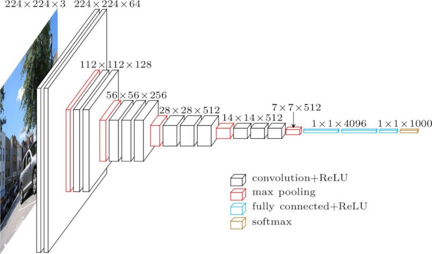
VGG-16 Architecture: Our input sizes were slightly different, but the layers were organized like above
Process
Data Manipulation and the Batch Spectrogram
Any good Data Scientist knows that preparation is 90% of the game, so I spent quite a bit of time arranging, labeling, and cleaning the data.
To train a VGG-16 there needs to be well-defined classes. The open-source sound data we chose came with .wav files with names such as “10120.wav”. This number is associated with a row value of the “1” column from an included .csv file. That same row tells you much more detailed information such as the sound source. There were around 10k samples a total of various lengths.
To accomplish the goal of organizing all of the files. I had to change the format of the .wav file to “sound_source + sample_number.wav”. As an example “10022.wav” is actually “Acoustic_guitar_22.wav”(this is the actual image in the header of the article). This was accomplished using Pandas. With Pandas, you can easily and non-recursively extract information into “column” based structures(i.e. DataFrames).
#in what directory are our audio files?
path = './Ambient_Audio'
path_csv = './Ambient_Audio/_test_post_competition_scoring_clips.csv'
#Read the files into an array audio_files
audio_files = glob(path + '/*.wav') #adds anthing with extension .wav

####Read the CSV for the title content
df = pd.read_csv(path_csv)
df2 = df[['label','fname']]
print(df.head())
print(df2.head())
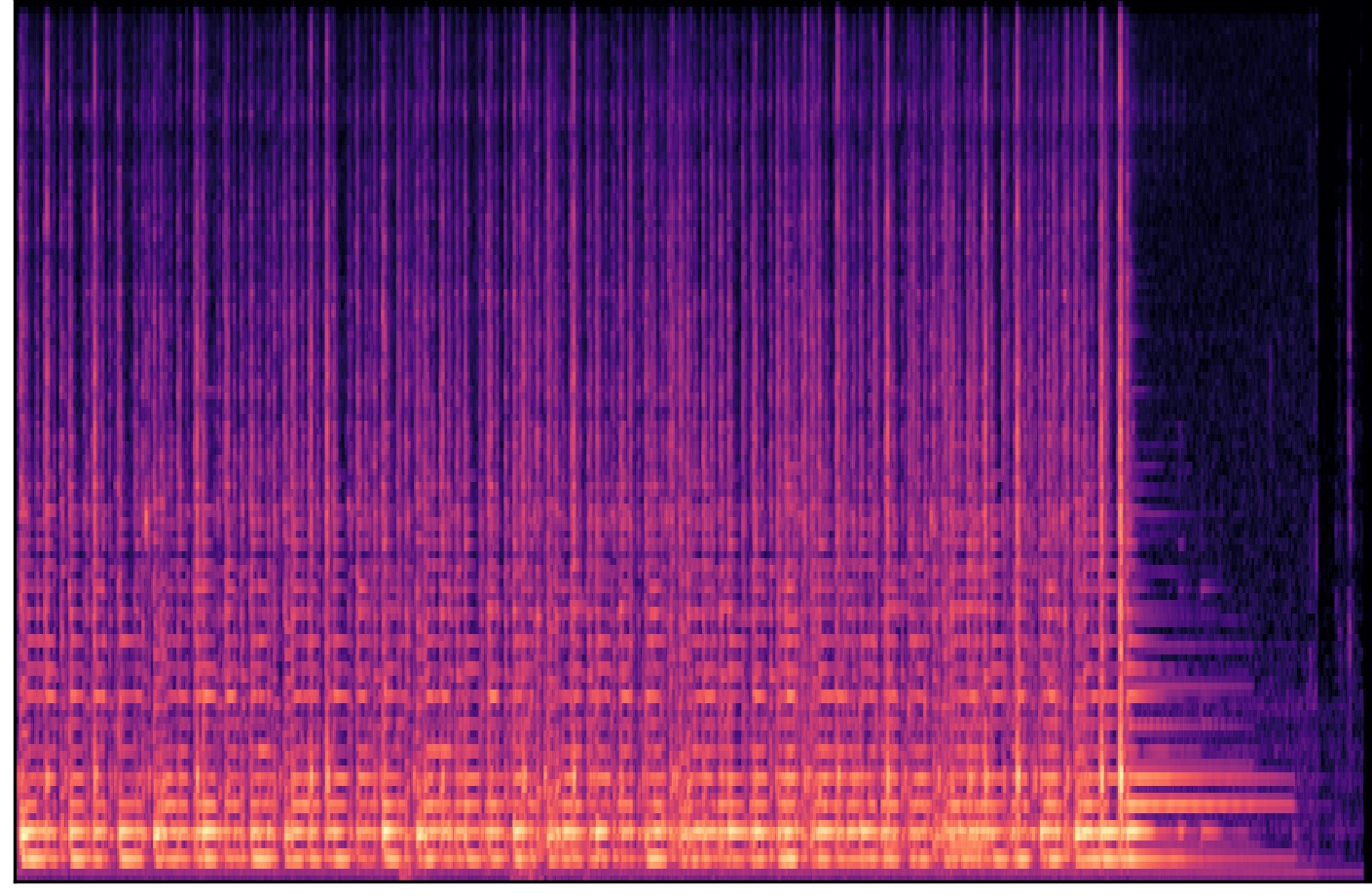
Once I had all of the “correct” names stored in a DataFrame, I used Librosa to convert all of the images into batch spectrograms form. Batch Spectrograms allow you to have time, power, and frequency information in one picture.

MEL Spectrogram: This picture is a long timeline of multiple weapon shots
#y refers to amplitude
#sr refers to sample rate
#load a specific file audio_files[i]
for i in range(len(audio_files)): #replace with length of
    y, sr = lr.core.load(audio_files[i])
    #where y is an array representing the audio time series
    #where sr is the sampling rate and a scalar

    #to find the magnitude spectrogram S
    S = lr.feature.melspectrogram(y=y, sr=sr)
    #extracts all of the mfcc from y and the sample rate
    #Takes the fast fourier transform I believe?
    S_dB = lr.power_to_db(S, ref =np.max)

        #open a second figure
    #plt.figure(i)
    lr.display.specshow(S_dB, sr=sr, fmax=44000)
    #x_axis = 'time', y_axis = 'mel',


    ###Attaching the file names to filenames######
    current_full_fname = audio_files[i]
    # pull just the last 8 elements of string also known as the label!
    #note that the .wav is also part of the label
    current_fname = current_full_fname[-12:]
    print(current_fname)
    ##See if that value is in the dataframe column 'label'
    df3 = df2.loc[df['fname'] == current_fname]
    final_fname = df3.iloc[0,0]


    plt.savefig( final_fname + '_'+ str(i)  + '_mel.jpg' , pad_inches = 0, bbox_inches='tight', dpi=300)
    #plt.title(final_fname)
    #add a title
Training on Super Computer Clusters
No worries, the following sections are not nearly as long as the data manipulation sections.
Through my sponsor, I was able to gain access to the Olympus supercomputing clusters at A&M to Train my model. The classes were chosen as:
- multiple_gunshots
- not_gunshots
- single_shots
Because my model has RGB coloring, it is helpful to normalize data to prevent huge networks, which may or may not converge. The images were normalized from ~ 900x1400 px to 244px by 159px. I used matplotlib to scale down the image to as small as I could make it before I felt the images were too similar.
Finally, I submitted everything in SLURM batch job files to Texas A&M, after installing all of the dependencies in my virtual python environment. There was a lot of obscure Linux to get everything to run, but in a few words, it was simply installing all dependencies and praying you didn’t mess up the batch file. It took a few tries before I understood the cluster.
At this point(Spring 2020), I had completed several ML projects already, so I had no issues with setting up or using TF(Tensorflow) or Keras. Below is just the layer and deployment code of one of the scripts.
model = tf.keras.models.Sequential([
    #Convolution and Max Pooling Layers
    tf.keras.layers.Conv2D(64, (3,3), activation = 'relu', input_shape = (244, 159, 3)),
    tf.keras.layers.Conv2D(64, (3,3), activation = 'relu'),
    tf.keras.layers.MaxPooling2D(2,2),
    #1st
    tf.keras.layers.Conv2D(128, (3,3), activation = 'relu'),
    tf.keras.layers.Conv2D(128, (3,3), activation = 'relu'),
    tf.keras.layers.MaxPooling2D(2,2),
    #2nd
    tf.keras.layers.Conv2D(256, (3,3), activation = 'relu'),
    tf.keras.layers.Conv2D(256, (3,3), activation = 'relu'),
    tf.keras.layers.Conv2D(256, (3,3), activation = 'relu'),
    tf.keras.layers.MaxPooling2D(2,2),
    #3rd
    tf.keras.layers.Conv2D(512, (3,3), activation = 'relu'),
    tf.keras.layers.Conv2D(512, (3,3), activation = 'relu'),
    tf.keras.layers.Conv2D(512, (3,3), activation = 'relu'),
    tf.keras.layers.MaxPooling2D(2,2),
    #4th
#    tf.keras.layers.Conv2D(512, (3,3), activation = 'relu'),
#    tf.keras.layers.Conv2D(512, (3,3), activation = 'relu'),
#    tf.keras.layers.Conv2D(512, (3,3), activation = 'relu'),
    tf.keras.layers.MaxPooling2D(2,2),
    #5th
    #Lines the neurons up for connecting to dense Layers
    tf.keras.layers.Flatten(),
    #Drops some hidden layers in order to reduce overfitting
    tf.keras.layers.Dropout(.5),

    #Dense Layer fully connected
    tf.keras.layers.Dense(4096, activation = 'relu'),
    tf.keras.layers.Dense(4096, activation = 'relu'),

    #Final 3 output layer Gunshot, Multiple Shots, or no gunshot
    tf.keras.layers.Dense(3, activation = 'softmax')
])


# ### Compiling and Testing the Model
#print the summary of our classes and of our model
model.summary()
#compile
model.compile(loss = 'categorical_crossentropy', optimizer='adam', metrics=['accuracy'])

#Try and save every checkpoint which is every epoch
checkpoint = ModelCheckpoint("404_ver1_best_model.h5",monitor='loss', verbose =1,save_best_only = True, mode= 'auto', period = 1)

#save the history and set verbose to 1 to see live printout, for now at 0 if running on background server
history = model.fit_generator(train_generator, epochs=1, validation_data = validation_generator, verbose = 1, callbacks = [checkpoint])


#Save the weights and biases of the trained model
model.save("404ver1.h5")
Model Layers: organized the classes’ file tree by hand.
Integration into an SBC
Generally, unless you have particular needs, the model weights and biases are saved to an “.h5” file. Once saved, this file can be used to pass appropriate inputs and predict a class. The problem for us was how to extract this prediction information “real-time”, and then display the prediction to an end user live constantly. And, to do this processing on a RPi4(Raspberry Pi 4)
To do this I generated a script that constantly makes predictions in 3-second intervals. Although this is not an ideal “live prediction” it was the best we could do with our power constraints on the RPi4.
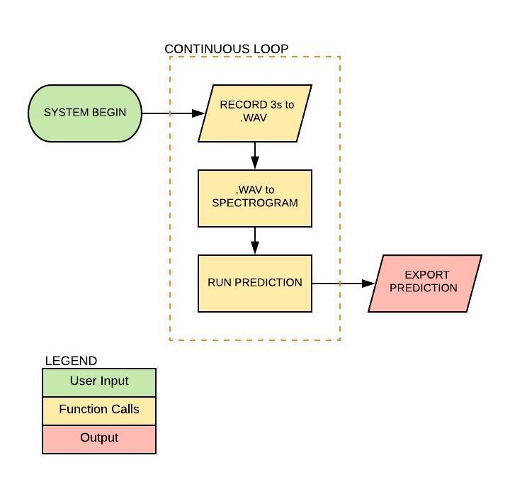
Continuous Prediction Loop: All the above are in a single script
# -*- coding: utf-8 -*-
"""
Created on Sat Feb 22 18:09:51 2020

@author: Daniel
"""
#---------------------RECORDING_RAW----------------
import sounddevice as sd
from scipy.io.wavfile import write

#---------------------SPECTROGRAM------------------
from glob import glob #For reading Files
import librosa as lr #For audio analysis
import librosa.display
from librosa import display

import numpy as np
import matplotlib.pyplot as plt #for plotting

#---------------------SPECTROGRAM------------------
from tensorflow.keras.models import load_model
from keras_preprocessing import image
from keras_preprocessing.image import load_img

model = load_model("404ver1.h5")

#How many times do you want to predict
for i in range(0,5):
    #Live Continous Prediction using Librosa and a Pretrained Model
    #Read in a audio signal and save it to .wav format
    #function 'record' takes in no inputs and outputs
    #the directory to where the .wav file is saved
    def record():
        #Our training audio is 44Khz
        fs = 44000
        #Let's say 3 seconds, we will pipeline
        seconds = 3

        #Record 3 seconds and save it
        current_recording = sd.rec(int(seconds*fs), samplerate = fs, channels = 2)
        #Wait until finished
        sd.wait()
        #Save as wav with approopriate size.
        write('last_3_seconds.wav', fs, current_recording)

        #Name the path of said recording as a string
        path_to_wav = './last_3_seconds.wav'
        return path_to_wav

    #After recording and saving the wav file, convert it into the
    #spectrogram image. 'spectro' has input path and output path_to_spectro
    def spectro(path_to_wav):
        #y refers to amplitude
        #sr refers to sample rate
        #load a specific file audio_files[i]
        y, sr = lr.core.load(path_to_wav)


        #extracts all of the mfcc from y and the sample rate
        #to find the magnitude spectogram S
        S = lr.feature.melspectrogram(y, sr=sr)
        #Takes the fast fourier transform I believe?
        S_dB = lr.power_to_db(S, ref=np.max)


        lr.display.specshow(S_dB,sr=sr, fmax=44000)
        plt.savefig('last_3_spectrogram.png', pad_inches = 0, bbox_inches='tight', dpi=300)
        plt.close()

        #Name the path of said figure
        path_to_spectro = './last_3_spectrogram.png'
        return path_to_spectro

    #After converting the wav to spectrogram, run an inference on it
    def predict(X):
        #Load images from file
        img = load_img(X , target_size = (1402,913) )
        #Turn into array for parsing
        img = image.img_to_array(img)

        #expand the dimensions horizontally, turn into one big line
        x = np.expand_dims(img, axis=0)
        #now stack it all vertically
        img = np.vstack([x])

        #use built model subfunctions to produce a prediction
        classes = model.predict_classes(img, verbose = 0)
        percent_classes = model.predict(img, verbose = 0)
        print(classes, '\n', percent_classes)
        return classes, percent_classes


    path_to_wav = record()
    path_to_spectro = spectro(path_to_wav)
    print(predict(path_to_spectro))
Finally, the prediction is displayed using RPi4’s camera module. Using some Picamera functions, I helped the other subsystems to display live predictions on a screen.
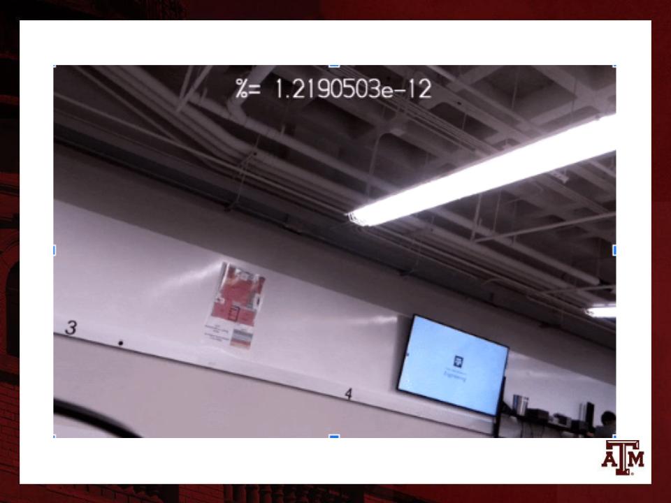
Live Camera Output: As you can see the probability of a gunshot was low at this point
Results
As a group, we scored an 89%, mainly because they have a policy of not giving As unless the project is sold to a company. As for the ML here are the metrics. The truth is more data and cleaner data is needed. Because of University and Safety policies we only collected around 100 or so samples of gunfire. Therefore the model had trouble finding patterns converging to gunshot classification. Although a high accuracy is shown, it is highly skewed by the not gunshot class. Simply put, I should have trained either on LSTM or by only having single shots as my only class.
Also unfortunate, Covid-19 interfered with finishing the project. Mainly this hindered mounting the system on a rover and transmitting information OTA(Over the Air) through Bluetooth. When progress was canceled, everything was “hardwired” still.
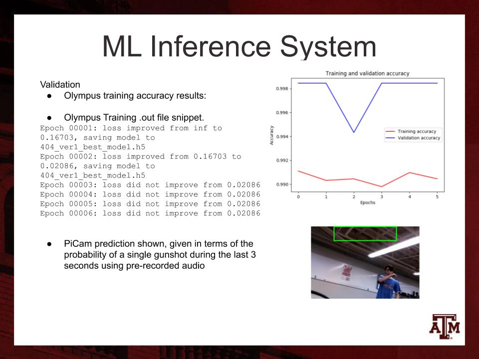
Metrics: Includes loss value checkpoints
Conclusion
In general terms, this is the project I am most proud of. And as it is my capstone, a high point in my college education. Using the latest technology in bleeding-edge labs at Texas A&M is always a pleasure. I would like to thank my, for now, unnamed sponsor, Samuel Beauchamp, and Jacob Beckham for being amazing partners.