Microstrip Simulation
Using MATLAB's GUI builder and Recursive methods
Project Specifications
This is a MATLAB and MATLAB app builder project. It was part of ECEN 445, an elective course in Applied Electromagnetics.
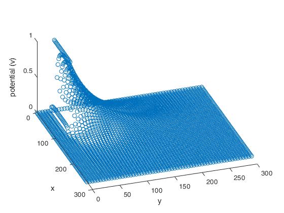
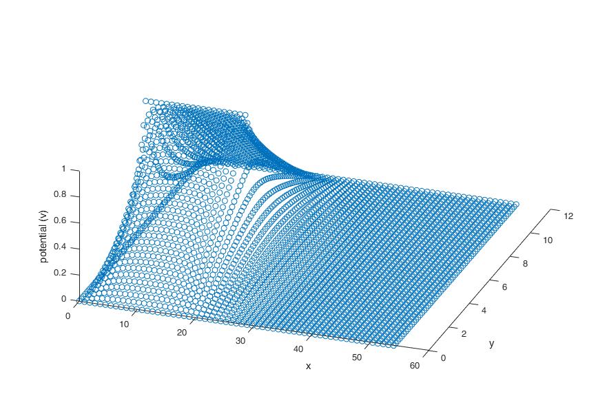
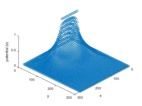
The mathematical concept is an exercise in recursive methods. There is a layout of nodes on an X and Y plane. The Z plane is the measure of Potential in volts.
In the middle, there is a simulated microstrip line that reaches about halfway into the viewable area. That theoretical line is of width 0 and has a 1-volt current running through it.
There is a perfect conductor wall the surrounds the area of study. The voltage of this wall is 0.
The Requirements:
-
Create a script that updated each node value, until the difference between the updated and previous nodes value was less than .001 Volts.
-
Create a UI that would allow a user to make a simulation with as many aspect ratios and nodes as they desired.
Process
Back-End
The voltage value of each node is affected by the nodes around it, described by an equation that contains the last value of the current node, and the current values of the nodes around it. Therefore this equation was put into a MATLAB script and called upon when needed. Note that this equation needs multiple iterations before a minimal difference is observed.
I wrapped that equation inside a function for calling as needed. Then with given inputs, I first create a grid, then use the said equation to update the nodes from top left to bottom right.
function [countIter, alpha, omega, cap] = FDSOR_Generation(a,b,d,w,n_a,n_b,e_r,threeD)
    %% SET PARAMETERS
    %Let's use a common denominator of 6 for d
    %test case number 1.
    %initial parameters

    f = uifigure;
    u = uiprogressdlg(f,'Title','Running FDSOR on Chosen Geometry', 'Message','Loading ','Cancelable','on');

    %convTol = .00001;%convergance tolerance
    convTol = .00001;

    wd = w / d;
    bd = b / d;
    aw = a / w;

    %horizontal distances
    h = a / n_a;

    %vertical distances
    k = b / n_b;

    %ratio
    alpha = h/k;

    %optimal relaxation
    omega = 2*(1 - (pi/sqrt(2))*sqrt(((1/n_a^2) + (1/n_b^2))));

    %% GENERATE BOX and STRIPLINE
    %Outputs will be the
    %optimal relax factor
    %The final capacitance
    %The plot of potentials

    %%% Generate Potentials %%%

    %First columns tracks X Boundary
    %Second columns tracks Y Boundary
    x = [0;a;a;0];
    y = [0;0;b;b];

    %Generate the boundary points
    %plot(x,y, 'k', 'Linewidth', 3);
    hold off %stiill need to superimpose points

    %Generate the stripline
    x= [0;w];
    y = [6,6];
    %plot(x,y, 'k', 'Linewidth',3)

    %% GENERATE NODES
    %x values go from 0 to the length 'a'
    %in intervals of 'h'
    xx = 0:h:a;

    %y values go from 0 to height 'b'
    %in intervals of k
    yy = 0:k:b;

    %use th meshgrid function to get an xy grid
    [X,Y] = meshgrid(xx,yy);
    %Each row is a copy of X
    %Each column is a copy of Y

    %pull the individual coordinates and store them
    %into columns X and Y
    PotCoord = [X(:),Y(:)];
    ZeroPots = zeros(size(PotCoord,1),1);
    PotCoord = [PotCoord,ZeroPots];

    %plot(PotCoord(:,1), PotCoord(:,2), 'o')

    %% GENERATE NODE POTENTIALS
    %initialze the 3rd col of PotCoord to 0
    %This is basically initizaling all the voltages to 0
    close all


        %We iterate through all but one "layer" of the boxes forms
        %this will maintain the outside nodes at zero always
    %     for jj = k:k:b-k
    %         for ii = h:h:a-h

    Residuals = zeros(1,size(PotCoord(:,1), 1));%Preallocate Residual

    Rmax = 1; %initialize the max residual for now ie 1 volt
    countIter = 0;%Count Iterator
    idxRes = 0;%Address Pointer of Residuals

    while (Rmax > convTol)
        if u.CancelRequested
            break
        end
        if countIter == 1000
            break
        end

        for jj = k:k:b-k
            for ii = h:h:a-h

                %Find the CURRENT Node Potential
                    %store all of the elements
                    %of PotCoord where the first column is
                    %our current x, and all the elemnents where the second
                    %column is our current y
                    %Extract the row into tmp
                try
                  tmpCurr = [ii,jj]; %what pt am I looking for
                  %find a row that closes matches that from my grid matrix
                  [~, idxCurrent] = ismembertol(tmpCurr, PotCoord(:,[1:2]), 'ByRows', true);
                  %store that row which is [x,y,potential]
                  tmpCurr = PotCoord(idxCurrent,:);
                  %Extract just the potential from that
                  CurrPot = tmpCurr(:,3);
                catch
                end
                try
                  tmpRight = [ii+h,jj];
                  [~, idxRight] = ismembertol(tmpRight, PotCoord(:,[1:2]), 'ByRows', true);
                  tmpRight = PotCoord(idxRight,:);
                  RightPot = tmpRight(:,3);
                catch
                  %If the above returns an empty, then you are outside the box
                  %therefore the potentials should be zero
                  RightPot = 0;
                end

                try
                  tmpLeft = [ii-h,jj];
                  [~, idxLeft] = ismembertol(tmpLeft, PotCoord(:,[1:2]), 'ByRows', true);
                  tmpLeft = PotCoord(idxLeft,:);
                  LeftPot = tmpLeft(:,3);
                catch
                  LeftPot = 0;
                end
                try
                  tmpAbove = [ii,jj+k];
                  [~, idxAbove] = ismembertol(tmpAbove, PotCoord(:,[1:2]), 'ByRows', true);
                  tmpAbove = PotCoord(idxAbove,:);
                  AbovePot = tmpAbove(:,3);
                catch
                  AbovePot = 0;
                end

                try
                  tmpBelow = [ii,jj-k];
                  [~, idxBelow] = ismembertol(tmpBelow, PotCoord(:,[1:2]), 'ByRows', true);
                  tmpBelow = PotCoord(idxBelow,:);
                  BelowPot = tmpBelow(:,3);
                catch
                  BelowPot = 0;
                end


                %Update the current potential
                %Here is function that finds the new potential
                R_p = FindNewPot(LeftPot,RightPot,AbovePot,BelowPot,e_r,alpha,tmpCurr);
                R_p = R_p - CurrPot;

                %Which point do we want to update? tmpCurr
                %find that row inside PotCoords and pull the index
                [~, idx] = ismembertol(tmpCurr, PotCoord, 'ByRows', true);

                %Now update that point with our new potential
                %Recall that the third column holds the potentials.
                PotCoord(idx,3) = CurrPot + omega * R_p;

                %Before we go on to the next node, we should check if our current
                %index is actually on the stripline i.e. ii <= w, and jj == d
                 if (tmpCurr(:,1) <= w) && (tmpCurr(:,2) == d)
                     PotCoord(idx,3) = 1;
                 end

                %Now we update the residuals
                %Residuals = [Residuals, R_p];
                idxRes = idxRes + 1;
                Residuals(idxRes) = R_p;
            end
        end
        %We check the residuals matrix to figure out when to stop iterating
        idxRes = 0;

        Rmax = max(Residuals);
        u.Message = 'Current Max Residual ' + string(Rmax);

        %Residuals = []; %clear Residuals
        countIter = countIter + 1;


    end
    %% PLOTTONG
    if threeD == 1
        figure
        plot3(PotCoord(:,1),PotCoord(:,2),PotCoord(:,3),'o');
        xlabel('x')
        ylabel('y')
        zlabel('potential (v)')
        savefig(string(n_a)+ string(countIter) + '.fig');
    end
    %% FIND CAPACITANCE
        nb = d - 3*k; %Bottom Left Y
        na = d + 3*k; %Top Left Y
        ns = d; %height of the stripline

        mr = [w + 3 * h]; %Right most plane

        %sum from 0 to mr in steps of h
        %you need two potentials at each point the node above and below
        %current (m, nb+ k) (nb - k)
        LatSums = 0;
        for ii = 0:h:mr
            %find the potntial above the contour nb
            AboveCBpot = [ii,nb+k];
            [~,idxAboveCBpot] = ismembertol(AboveCBpot,PotCoord(:,[1:2]),'ByRows',true);
            A = PotCoord(idxAboveCBpot,3);

            %find the potential below the contour nb
            BelowCBpot = [ii,nb-k];
            [~,idxBelowCBpot] = ismembertol(BelowCBpot,PotCoord(:,[1:2]),'ByRows',true);
            B = PotCoord(idxBelowCBpot,3);

            %find the potntial above the contour na
            AboveCApot = [ii,na+k];
            [~,idxAboveCApot] = ismembertol(AboveCApot,PotCoord(:,[1:2]),'ByRows',true);
            C = PotCoord(idxAboveCApot,3);

            %find the potential below the contour na
            BelowCApot = [ii,na-k];
            [~,idxBelowCApot] = ismembertol(BelowCApot,PotCoord(:,[1:2]),'ByRows',true);
            D = PotCoord(idxBelowCApot,3);

            %Find the lateral capacitance a this locatation
            %Sum them up
            LatSums = LatSums + (e_r*(A-B) + (C-D));
        end

        VertSumBottom = 0;
        for ii = nb:k:ns
            LeftCPot = [mr+h, ii];
            [~,idx] = ismembertol(LeftCPot,PotCoord(:,[1:2]),'ByRows',true);
            A = PotCoord(idx,3);

            RightCpot = [mr-h, ii];
            [~,idx] = ismembertol(RightCpot,PotCoord(:,[1:2]),'ByRows',true);
            B = PotCoord(idx,3);

            VertSumBottom = VertSumBottom + (e_r*(A) - (B));
        end

        VertSumTop = 0;
        for ii = ns:k:na
            LeftCPot = [mr+h, ii];
            [~,idx] = ismembertol(LeftCPot,PotCoord(:,[1:2]),'ByRows',true);
            A = PotCoord(idx,3);

            RightCpot = [mr-h, ii];
            [~,idx] = ismembertol(RightCpot,PotCoord(:,[1:2]),'ByRows',true);
            B = PotCoord(idx,3);

            VertSumTop = VertSumTop + ((A) - (B));
        end

        cap = -1* (alpha*(LatSums) + (alpha^-1)*(VertSumBottom + VertSumTop));
    %% SAVE WORKSPACE
    save(string(n_a)+ string(countIter) + '.mat')
    %% UPDATE POTENTIAL FUNCTION
    function NewPot = FindNewPot(LeftPot,RightPot,AbovePot,BelowPot,e_r,alpha,tmpCurr)
    %First we should check if we are inside interface or not.
         if (tmpCurr(:,2) <= d)
             %e_r should be the user input
         else
             e_r = 1;
         end
        A =   (2*(1+alpha^2))^-1;
        B = (2*alpha^2)/(1+e_r);
        NewPot = A*(LeftPot + RightPot + B*(AbovePot + e_r*BelowPot));
    end
end
Front-End
Using MATLAB’s app builder and API like interface, I created an interface for a user to custom make a simulation. The main challenge was connecting this to the script that ran the simulation. Secondary, but still as difficult was making sure that the user ran the program correctly. To do this, I used button locks, indicator lights, warning messages, prompts, and more to make it as easy as possible.
I also stuck to a linear methodology of design, meaning I directed the user linearly. Finally, once a simulation was started, I indicated how many iterations were done, and the current tolerance level as a way of indicating how long it might run. Tolerance in this case meaning the biggest change that was made from one iteration to another from all the nodes. Once this was less than .001 Volts, the simulation was finished.
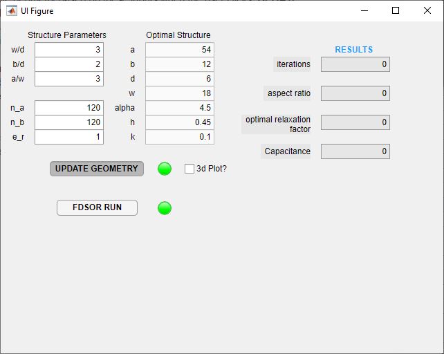
User Interface UI/UX:
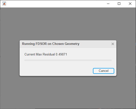
Live Simulation: Residual is also known as tolerance
Conclusion
While receiving an A was great, my biggest takeaway from this project was a deep understanding of the workflow needed to build a MATLAB UI, as well as plenty of practice with MATLAB itself.
Once the simulation was complete, a 3d plot was generated if so desired.
Simulation: With different parameters