Solar Power: Linear Regression Utility
Using Python's GUI builder and Tensorflow to make ML accessible. Creating a tool to estimate the effect of Solar Panel installations

Project Specifications
This was a completely optional project for the Data Science for Energy and Power class at Texas A&M. In addition to machine learning, this class focused on time predictive techniques and methodology such as ARMA, SVD, and K-means.
As many consumers begin to move to solar, it is hard to accurately measure the impact of the number of panels vs the environmental benefits a solar array creates. Many companies might stretch the truth about efficacy, while others may be more conservative in their estimates.
Therefore, the goal was to create a predictive model, that taking an input of solar panels to be installed (consumer panels have a standard size), could predict the carbon offset in metric tons of an installation. The model gets its prediction not by some set formula, but from a trained linear regression on the data provided by Google’s Project Sunroof
A secondary goal was to make this prediction tool user friendly, which involved creating a GUI that would allow anyone to see predictions.
Process
The first process is to obtain the data and to extrapolate the things that I need. Here is a snippet of the original table. It is organized by cities.
| region_name | state_name | lat_max | lat_min | lng_max | lng_min | lat_avg | lng_avg | yearly_sunlight_kwh_kw_threshold_avg | count_qualified | percent_covered | percent_qualified | number_of_panels_n | number_of_panels_s | number_of_panels_e | number_of_panels_w | number_of_panels_f | number_of_panels_median | number_of_panels_total | kw_median | kw_total | yearly_sunlight_kwh_n | yearly_sunlight_kwh_s | yearly_sunlight_kwh_e | yearly_sunlight_kwh_w | yearly_sunlight_kwh_f | yearly_sunlight_kwh_median | yearly_sunlight_kwh_total | carbon_offset_metric_tons | existing_installs_count |
|---|---|---|---|---|---|---|---|---|---|---|---|---|---|---|---|---|---|---|---|---|---|---|---|---|---|---|---|---|---|
| NULL | Pennsylvania | 40.70188 | 40.61294 | -75.4622 | -75.5461 | 40.65035 | -75.4958 | 985.15 | 7673 | 98.72285 | 84.84078 | 39701 | 113097 | 83193 | 87582 | 203964 | 32 | 527537 | 8 | 131884.3 | 10025162 | 35149706 | 23041858 | 24541877 | 59927475 | 9215.539 | 1.53E+08 | 97025.99 | 11 |
| NULL | NULL | 32.55156 | 32.54226 | -116.92 | -117.03 | 32.54845 | -116.957 | 1300.5 | 2 | 100 | 66.66667 | 13 | 18 | 0 | 0 | 0 | 13 | 31 | 3.25 | 7.75 | 4745.559 | 7692.078 | 0 | 0 | 0 | 5209.465 | 12437.64 | 0 | 0 |
| Aberdeen | North Carolina | 35.18396 | 35.05361 | -79.3885 | -79.5383 | 35.1436 | -79.4247 | 1083.75 | 1078 | 86.0984 | 71.62791 | 3248 | 16681 | 13821 | 12775 | 92404 | 38 | 138929 | 9.5 | 34732.25 | 916858.5 | 5550471 | 4255421 | 3855701 | 30274566 | 11665.38 | 44853017 | 26330.81 | 0 |
| Abilene | Texas | 32.61433 | 32.23666 | -99.5896 | -100.086 | 32.43502 | -99.7507 | 1252.411 | 42802 | 97.87507 | 93.67504 | 172303 | 586619 | 403010 | 557991 | 1718095 | 42 | 3438018 | 10.5 | 859504.5 | 56039759 | 2.34E+08 | 1.4E+08 | 2.04E+08 | 6.44E+08 | 15695.83 | 1.28E+09 | 621366.8 | 25 |
First, I got rid of all of the nulls and pulled the two columns I was interested in… number_of_panels_total and carbon_offset_metric_tons. I retrospect, I should have checked to see how many nulls there were, and if this was an appropriate measure to take.
| number_of_panels_total | carbon_offset_metric_tons |
|---|---|
| 527537 | 97025.99147 |
| 31 | 0 |
| 138929 | 26330.80621 |
| 3438018 | 621366.8494 |
| 175853 | 21479.14411 |
| 170469 | 31333.36638 |
| 31219 | 6075.026699 |
I plot this against each-other to see the relationship (cover picture)
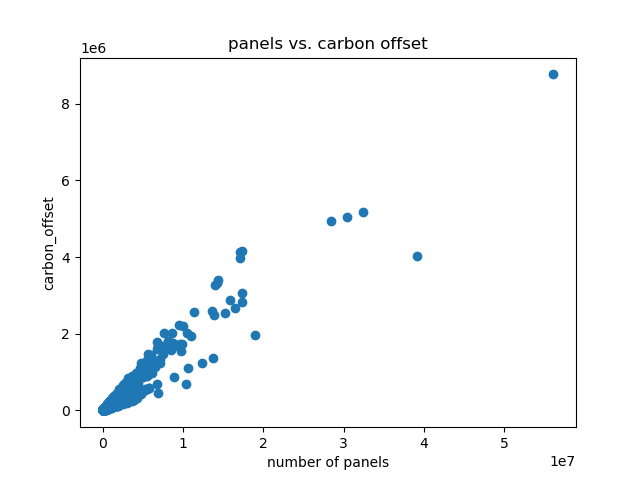
Relationship between number of panels and carbon offset.
The model
Using these two columns, I used Numpy, Keras, and TensorFlow to create a linear regression model. The code below is almost guided by the TF docs. It probably would have had an easier implementation just making my own, but the benefit of this code is that you could associate on output with multiple inputs, which again, I didn’t need.
import matplotlib.pyplot as plt
import numpy as np
import pandas as pd

import tensorflow as tf
from tensorflow import keras
from tensorflow.keras import layers

import tensorflow_docs as tfdocs
import tensorflow_docs.modeling

import tensorflow_docs.plots
from tensorflow.keras.models import load_model

#import the data from an excel/csv file
myFile  = pd.read_csv(r'E:\Daniel\Documents\_TAMU\_SPRING 2020\ECEN_489_POWER\_Solar_Project\city.csv', encoding = 'utf-8')
#turn the imported data into a dataframe
df1 = pd.DataFrame(myFile)

#extract the carbon offset datak
carbon_offset = df1[['carbon_offset_metric_tons']]
#extract the region data
region = df1[['region_name']]
#extract the number of panels
panels = df1[['number_of_panels_total']]


# combine carbon offset and panel data, drop nan columns
data_set = pd.concat([panels,carbon_offset], axis = 1)
data_set = data_set.dropna()

#Split the data
train_dataset = data_set.sample(frac=.8, random_state=0)
test_dataset = data_set.drop(train_dataset.index)


#set carbon offset as the Y output
Y_train = train_dataset.pop('carbon_offset_metric_tons')
Y_test = test_dataset.pop('carbon_offset_metric_tons')

#normalization
norm_train_dataset = (train_dataset-train_dataset.mean())/train_dataset.std()
norm_test_datatest = (test_dataset-train_dataset.mean())/train_dataset.std()
norm_Y_train = (Y_train-Y_train.mean())/Y_train.std()
norm_Y_test = (Y_test-Y_test.mean())/Y_test.std()


print("mean X = " + str(train_dataset['number_of_panels_total'].mean()))
print("std X = " + str(train_dataset['number_of_panels_total'].std()))

print("std Y= " +  str(Y_train.std()) )
print("mean Y= " +  str(Y_train.mean()) )

plt.scatter(data_set[['number_of_panels_total']], data_set[['carbon_offset_metric_tons']])
plt.title('panels vs. carbon offset')
plt.ylabel('carbon_offset')
plt.xlabel('number of panels')
plt.savefig('panels_v_carbon.png')
plt.show()

print(train_dataset.head(10))
#MODEL DEFINITIONS
def build_model():
  model = tf.keras.models.Sequential([
    tf.keras.layers.Dense(64, activation='relu', input_shape=[len(train_dataset.keys())]),
    tf.keras.layers.Dense(64, activation='relu'),
    tf.keras.layers.Dense(1)
  ])

  optimizer = tf.keras.optimizers.RMSprop(0.001) #learning rate

  model.compile(loss='mse',
                optimizer=optimizer,
                metrics=['mae','mse'])
  return model

model = build_model()#build the structure of the model


EPOCHS = 1000 #train the model 1000 iterations
stop_training = keras.callbacks.EarlyStopping(monitor='val_loss', patience=50)

history = model.fit(
  norm_train_dataset, norm_Y_train,
  epochs=EPOCHS, validation_split = 0.2, verbose=0,
  callbacks=[stop_training, tfdocs.modeling.EpochDots()])

#model.save('solar_model.h5')

#evaluate the model using the testing set
loss, mae, mse= model.evaluate(norm_test_datatest,norm_Y_test,verbose=2)
print(str(mae))

#use history function to plot accuracy
train_acc = history.history['mae']
val_acc = history.history['val_mae']

epochs = range(len(train_acc))

plt.plot(epochs, train_acc, 'r', label='Mean Absolute Error')
plt.title('Error Decrease per Epoch')
plt.legend(loc=0)
plt.xlabel('Epochs')
plt.ylabel('MAE')
plt.savefig('Loss_Metrics.png')
plt.show()
The GUI
Once I had the produced h5 model, I used Tkinter to create the python application.
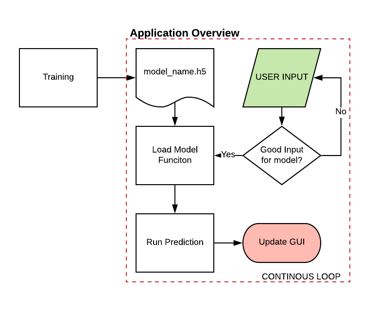
Overview of Solar Panel app
from tkinter import *

import matplotlib.pyplot as plt
import numpy as np
import pandas as pd

import tensorflow as tf
from tensorflow import keras
from tensorflow.keras import layers

import tensorflow_docs as tfdocs
import tensorflow_docs.modeling
import tensorflow_docs.plots

#Import the script for loading a module
from load_model import load_solar_model
#The input from user requires some preprocessing
def prep_user_input(txt_in):
    txt_cleaned = ''.join(i for i in txt_in if (i.isdigit() or i == '.'))

    try:
        new_text = float(txt_cleaned)
    except ValueError:
        print('ERROR: Please enter a real numerical value!')
    predict_input = np.array([new_text])
    predict_input = predict_input[:1]

    # print(predict_input)
    return predict_input, txt_cleaned


#make all of my fonts the same
myfont = "Circular Std bold"
#Where is the model currently saved
mypath = 'E:\Daniel\Documents\_TAMU\_SPRING 2020\ECEN_489_POWER\_Solar_Project\CodeFiles\solar_model.h5'

#open the main window loop
window = Tk()
window.title("Solar Panels Carbon Offset Estimation App")
#window.geometry('700x700')

#BUTTON CLICKED ACTION
def run_prediction():
    #when button is clicked, gather what was in the text field
    number_of_panels = txt.get()

    #prep it through formatting for loading to the machine learning model
    predict_input, txt_cleaned = prep_user_input(number_of_panels)

    #show the formatted array input to the user
    b.configure(text="Calculating Carbon Offset for: " + txt_cleaned + " panels") #change text to calulating
    print(predict_input)

    #send it to load_model for evaluating
    out_prediction = load_solar_model(predict_input, mypath)

    #Show the prediction
    pred_txt.configure(text = 'Predicted Carbon Offset(metric tons): ' + np.array2string(out_prediction))
    #.....


#DECRIPTIVE TEXT
b = Label(window, text ='Enter number of solar panels:', font=(myfont,10))
b.grid(column=1, row=0)

#TEXT INPUT
txt = Entry(window, width = 50)
txt.grid(column= 1, row = 1)

#MAIN CALCULATE BUTTON
calculate_btn = Button(window, text = "PREDICT", command = run_prediction, font=(myfont,10))
calculate_btn.grid(column = 1, row = 2)

#SHOW THE OUTPUT FOR GIVEN PREDICTION
pred_txt = Label(window, text ='Predicted carbon offset: ', font = (myfont,10))
pred_txt.grid(column = 1, row = 3)

window.mainloop()
import matplotlib.pyplot as plt
import numpy as np
import pandas as pd

import tensorflow as tf
from tensorflow import keras
from tensorflow.keras import layers
from tensorflow.keras.models import load_model

import tensorflow_docs as tfdocs
import tensorflow_docs.modeling
import tensorflow_docs.plots

def load_solar_model(number_panels, myPath):
    #load saved model
    carbon_model = load_model(myPath)
    #evaluate input into your model
    est_carbon_offset = carbon_model.predict(number_panels)
    return est_carbon_offset

#This will go into further parameters
#file path is user determined
# filepath = 'E:\Daniel\Documents\_TAMU\_SPRING 2020\ECEN_489_POWER\_Solar_Project\CodeFiles\solar_model.h5'
# number_panels = np.array([.3])
# cb_off = load_solar_model(number_panels[:1], filepath)

# print(number_panels)
# print(str(cb_off))
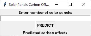
GUI before entry
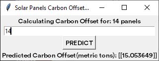
GUI after entry
Conclusion
Using MAE as our loss value because the values were so large MSE might be a bad measure, we reached 92% accuracy or 8% MAE. Generally, the project was a success. In the future, I would like to develop this further for municipalities that may be looking at solar power.